Blockmodeling • signnet

This vignette describes the two implemented methods for blockmodeling in signed networks.

library(igraph)
library(signnet)

Traditional Blockmodeling

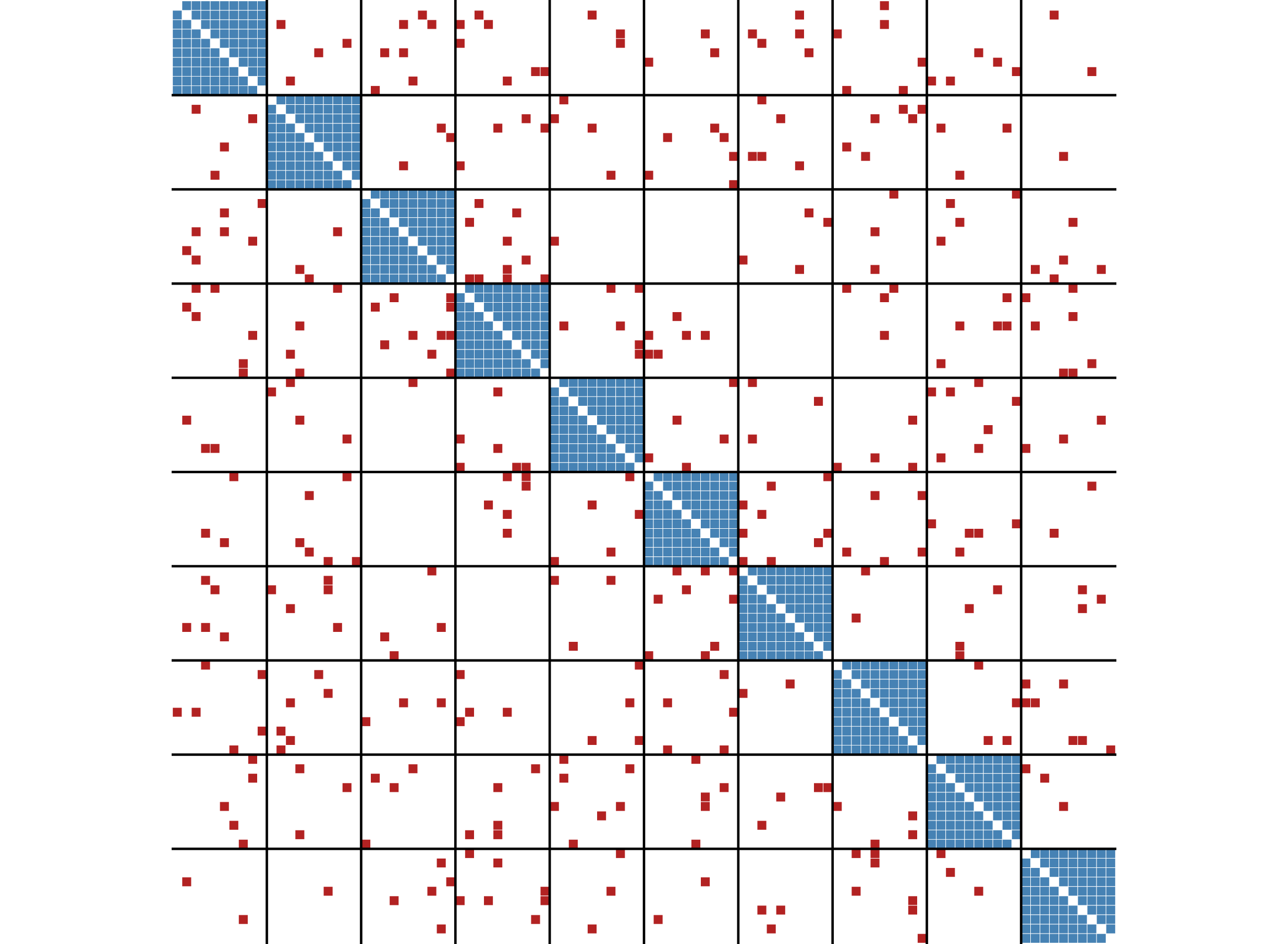
In signed blockmodeling, the goal is to determine k blocks of nodes such that all intra-block edges are positive and inter-block edges are negative. In the example below, we construct a network with a perfect block structure with sample_islands_signed(). The network consists of 10 blocks with 10 vertices each, where each block has a density of 1 (of positive edges). The function signed_blockmodel() is used to construct the blockmodel. The parameter k is the number of desired blocks. alpha is a trade-off parameter. The function minimizes $P(C)=\alpha N+(1-\alpha)P$ , where $N$ is the total number of negative ties within blocks and $P$ be the total number of positive ties between blocks.

g <- sample_islands_signed(10,10,1,20)
clu <- signed_blockmodel(g,k = 10,alpha = 0.5)
table(clu$membership)
#> 
#>  1  2  3  4  5  6  7  8  9 10 
#> 10 10 10 10 10 10 10 10 10 10
clu$criterion
#> [1] 0

The function returns a list with two entries. The block membership of nodes and the value of $P(C)$ .

The function ggblock() can be used to plot the outcome of the blockmodel (ggplot2 is required).

ggblock(g,clu$membership,show_blocks = TRUE)

If the parameter annealing is set to TRUE, simulated annealing is used in the optimization step. This generally leads to better results but longer runtimes.

data("tribes")
set.seed(44) #for reproducibility

signed_blockmodel(tribes,k = 3,alpha=0.5,annealing = TRUE)
#> $membership
#>  [1] 1 1 2 2 3 2 2 2 3 3 2 2 3 3 1 1
#> 
#> $criterion
#> [1] 2
signed_blockmodel(tribes,k = 3,alpha=0.5,annealing = FALSE)
#> $membership
#>  [1] 1 1 2 2 3 2 2 2 3 3 2 2 3 3 1 1
#> 
#> $criterion
#> [1] 2

Generalized Blockmodeling

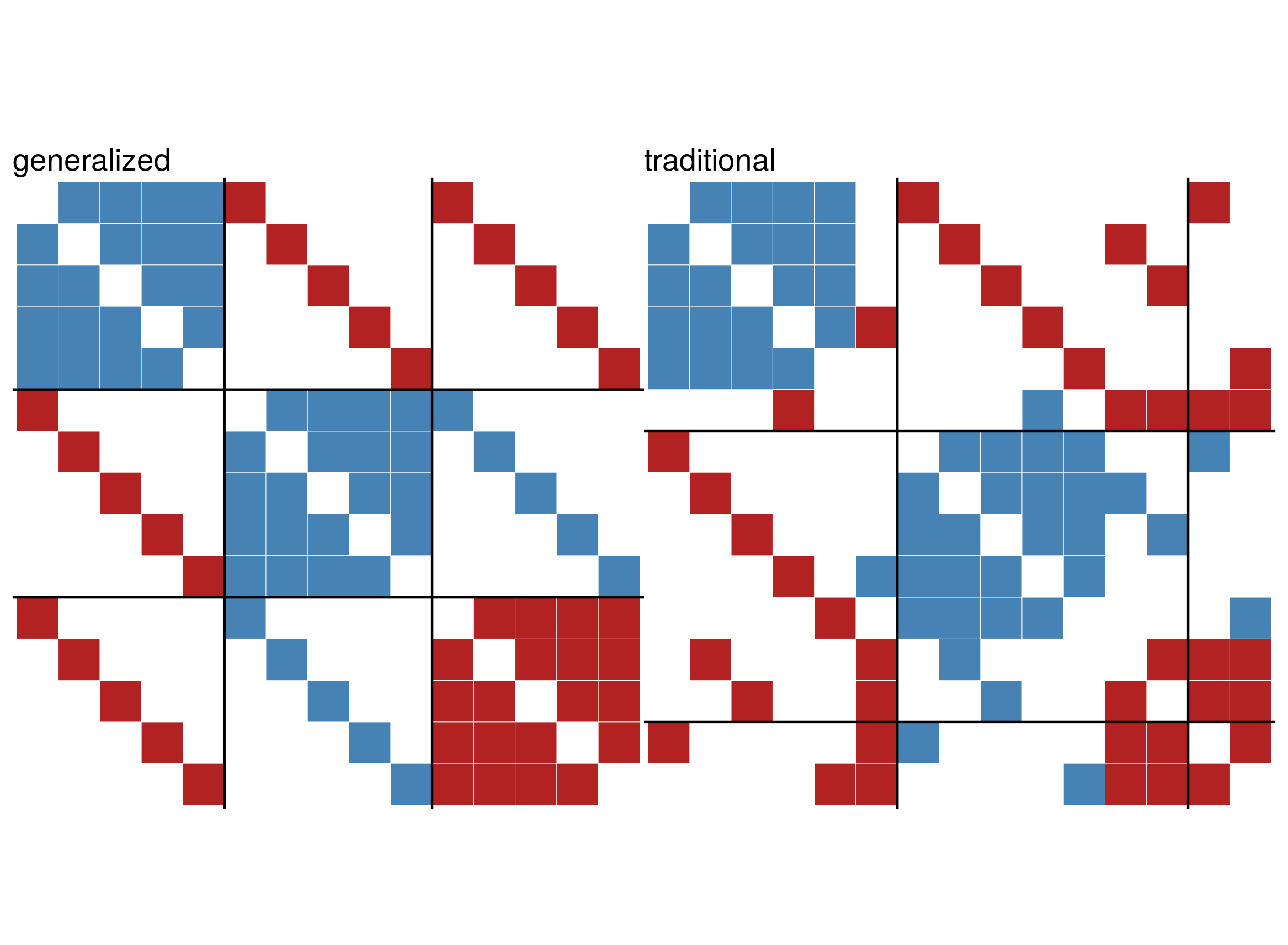
The function signed_blockmodel() is only able to provide a blockmodel where the diagonal blocks are positive and off-diagonal blocks are negative. The function signed_blockmodel_general() can be used to specify different block structures. In the below example, we construct a network that contains three blocks. Two have positive and one has negative intra-group ties. The inter-group edges are negative between group one and two, and one and three. Between group two and three, all edges are positive.

g1 <- g2 <- g3 <- graph.full(5)

V(g1)$name <- as.character(1:5)
V(g2)$name <- as.character(6:10)
V(g3)$name <- as.character(11:15)

g <- Reduce("%u%",list(g1,g2,g3))
E(g)$sign <- 1
E(g)$sign[1:10] <- -1
g <- add.edges(g,c(rbind(1:5,6:10)),attr = list(sign=-1))
g <- add.edges(g,c(rbind(1:5,11:15)),attr = list(sign=-1))
g <- add.edges(g,c(rbind(11:15,6:10)),attr = list(sign=1))

The parameter blockmat is used to specify the desired block structure.

set.seed(424) #for reproducibility
blockmat <- matrix(c(1,-1,-1,-1,1,1,-1,1,-1),3,3,byrow = TRUE)
blockmat
#>      [,1] [,2] [,3]
#> [1,]    1   -1   -1
#> [2,]   -1    1    1
#> [3,]   -1    1   -1

general <- signed_blockmodel_general(g,blockmat,alpha = 0.5)
traditional <- signed_blockmodel(g,k = 3,alpha = 0.5,annealing = TRUE)

c(general$criterion,traditional$criterion)
#> [1] 0 6

References

Doreian, Patrick, and Andrej Mrvar. 1996. “A Partitioning Approach to Structural Balance.” Social Networks 18 (2): 149–68.

Doreian, Patrick, and Andrej Mrvar. 2009. “Partitioning Signed Social Networks.” Social Networks 31 (1): 1–11.

Doreian, Patrick, and Andrej Mrvar. 2015. “Structural Balance and Signed International Relations.” Journal of Social Structure 16: 1.