library(tidygraph)
library(networkdata)23 Descriptive Network Analysis
This chapter revisits the descriptors introduced in the Descriptive part — centrality, community structure, and the assortment of node- and edge-level measures — through tidygraph. The point is not to teach the descriptors again but to show how the same computations translate into pipeable mutate() calls on an activated node or edge table. Cross-references to the original treatment in Centrality and Cohesive Subgroups are given where they help.
23.1 Packages Needed for this Chapter
data("flo_marriage")
flo_tidy <- as_tbl_graph(flo_marriage)
23.2 Centrality
Centrality indices live in the centrality_*() function family. The family covers everything implemented in igraph — degree, closeness, betweenness, eigenvector, PageRank, Katz, hub and authority scores — together with the richer catalogue exposed by the netrankr package. Every function in the family shares the same calling convention: no graph argument, no vertex argument, just the name. Each one reads the currently active graph implicitly and returns a vector the length of the active table, which is what makes them slot straight into mutate() alongside any other derived column. Figure 23.1 combines degree and betweenness in a single pipeline and maps them to node size and fill.
flo_tidy |>
  activate("nodes") |>
  mutate(
    degree = centrality_degree(),
    betweenness = centrality_betweenness()
  ) |>
  ggraph("stress", bbox = 10) +
  geom_edge_link0(edge_color = "black") +
  geom_node_point(
    shape = 21,
    aes(size = degree, fill = betweenness)
  ) +
  geom_node_text(aes(label = name)) +
  scale_fill_gradient(low = "#104E8B", high = "#CD2626") +
  scale_size(range = c(4, 10)) +
  theme_graph()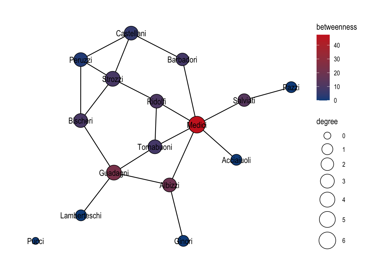
A practical tip: because every function starts with the same prefix, typing centrality_ in most IDEs and pressing Tab is the fastest way to browse what is available without consulting the help pages first.
23.3 Clustering
Community detection algorithms are exposed through the parallel group_*() family: group_louvain, group_infomap, group_edge_betweenness, group_walktrap, group_leading_eigen, group_fast_greedy, group_label_prop, group_spinglass, group_components, group_biconnected_component, and a few more. Each returns an integer membership vector the length of the node table, which means the idiomatic usage is mutate(community = as.factor(group_*())) — coerce to factor so the result becomes a natural input to a fill or color aesthetic.
We illustrate the pattern on a random graph with planted community structure, generated with play_islands() (the tidygraph equivalent of igraph::sample_islands()). The Louvain partition recovered on that graph is shown in Figure 23.2.
play_islands(4, 12, 0.8, 4) |>
  mutate(community = as.factor(group_louvain())) |>
  ggraph(layout = "stress") +
  geom_edge_link0() +
  geom_node_point(aes(fill = community), shape = 21, size = 6) +
  theme_graph()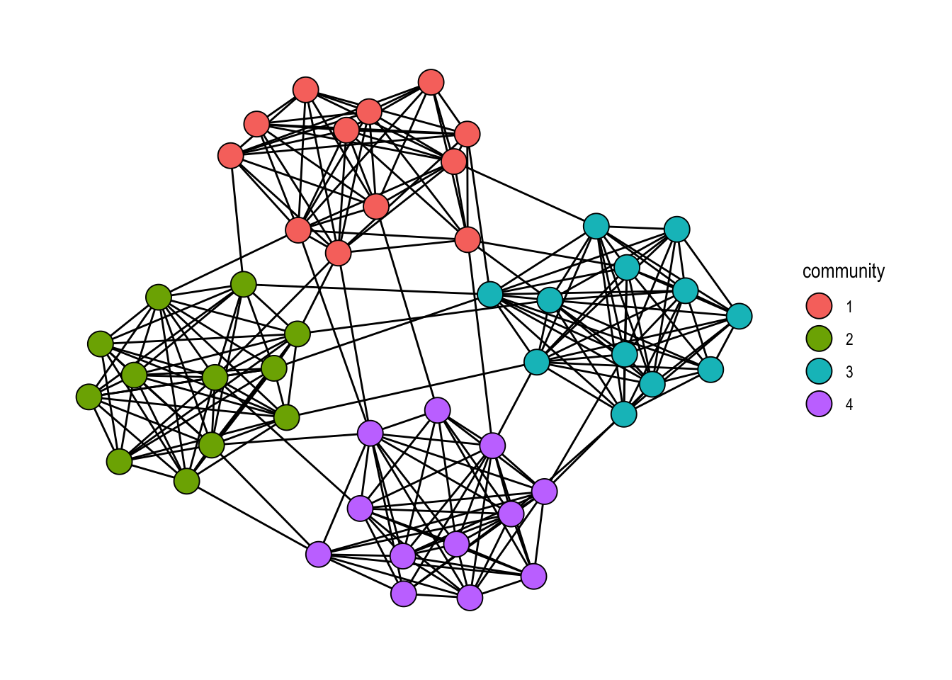
play_islands(). Node fill encodes the recovered community membership.
A frequent follow-up is to color edges by community — one color when an edge stays inside a cluster, another when it bridges two clusters. The way to do this is to propagate the node-level community attribute into the edge table using .N()[from] and .N()[to], which look up the community of each edge’s endpoints. If they match, the edge is intra-community; otherwise, we mark it as a bridge. Figure 23.3 shows the resulting picture.
play_islands(4, 12, 0.8, 4) |>
  mutate(community = as.factor(group_louvain())) |>
  activate("edges") |>
  mutate(
    community = as.factor(ifelse(
      .N()$community[from] == .N()$community[to],
      .N()$community[from],
      5
    ))
  ) |>
  ggraph(layout = "stress") +
  geom_edge_link0(aes(edge_color = community), show.legend = FALSE) +
  geom_node_point(aes(fill = community), shape = 21, size = 6) +
  scale_fill_brewer(palette = "Set3") +
  scale_edge_color_brewer(palette = "Set3") +
  theme_graph(background = "grey88")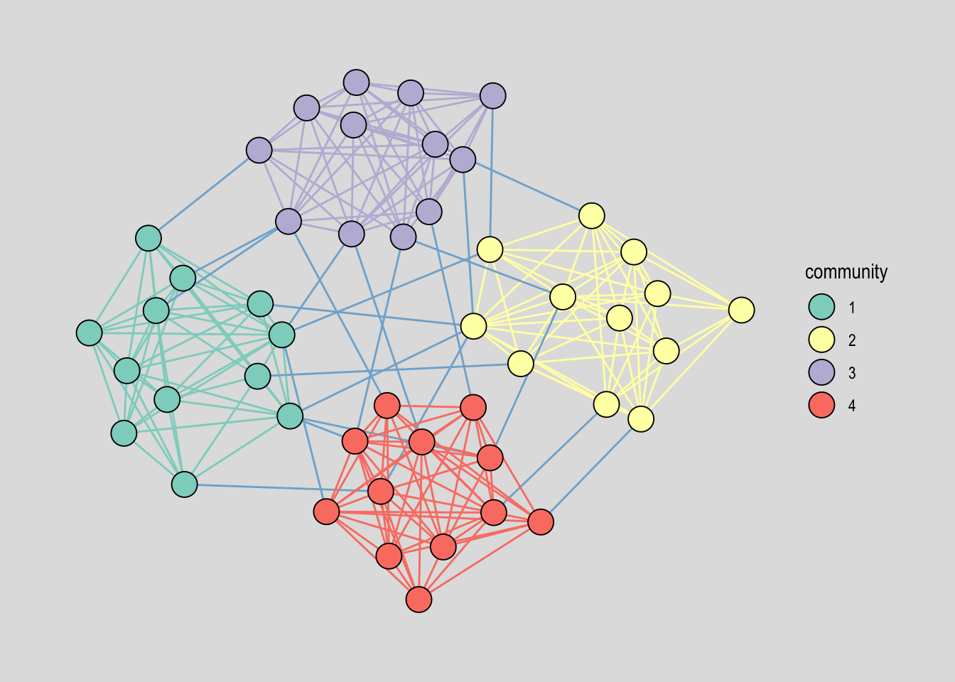
23.4 Other node or edge level functions
Beyond centrality and grouping, tidygraph harmonises a long list of node- and edge-level measures behind two mirror-image function families: node_*() returns a vector of length vcount(), and edge_*() returns a vector of length ecount(). Which family you reach for is determined by which table you have activated. The families cover distance (node_distance_to, node_distance_from, node_eccentricity), local structure (node_triangles, node_coreness, node_local_transitivity), and tests on edges (edge_is_loop, edge_is_multiple, edge_is_mutual, edge_is_incident), among many others. As with the centrality and group families, typing node_ or edge_ at the prompt and pressing Tab gives the full list.
The example below combines one of each: on nodes, the geodesic distance to the Medici family; on edges, a flag indicating whether the edge is incident to the Medici. Activating each table in turn keeps both computations in a single pipeline, and the result is shown in Figure 23.4.
flo_tidy |>
  activate("nodes") |>
  mutate(dist2Medici = node_distance_to(nodes = 9)) |>
  activate("edges") |>
  mutate(edge2Medici = edge_is_incident(9)) |>
  ggraph("stress") +
  geom_edge_link0(aes(edge_color = edge2Medici)) +
  geom_node_point(aes(fill = dist2Medici), size = 9, shape = 21) +
  theme_graph()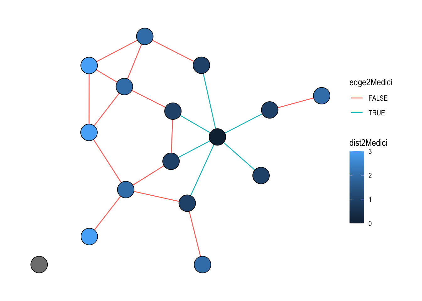
The node id 9 refers to the Medici, which happens to be the ninth row of the node table. Passing the index directly is the quickest way when you already know the position; for a name-based lookup you can equally write nodes = which(.N()$name == "Medici").